What Is Moving Average Filter In Computer Vision

[CV] 1. Prototype Processing Basic: Linear Filters

Computer Vision (CV) consists of various research areas, such equally filters, edge detection, segmentation, feature extraction & matching, object detection, 3D reconstruction and so on.

In this article, and in hereafter, I aim to go through the fundamental ideas of all mentioned topics, merely equally the showtime step, we will start with the basics of image processing, namely the filters.

1. What is Filter?

As its proper name implies, the purpose of filters is to filter out some unnecessary components (in other words, the noise) or to excerpt some structures underlying the paradigm.

**Figure ane. images with different level of noise (left panel) and extracted structure (edge) from the original prototype (right panel) from** **[i]** , **[2]**

Out of many types of filter, we will accept a look at linear and non-linear filters. More than specifically, our focus is on what are they, how they work, why they are benign. Only earlier getting into these topics, we first need to know what is noise.

2. Noise

Noise is unwanted and unexpected signals in images. It distorts the original image by introducing a random variation of brightness, illumination or colour information into the image.

Commonly known types of noise are as follows: Salt & pepper, Impulse and Gaussian noise.

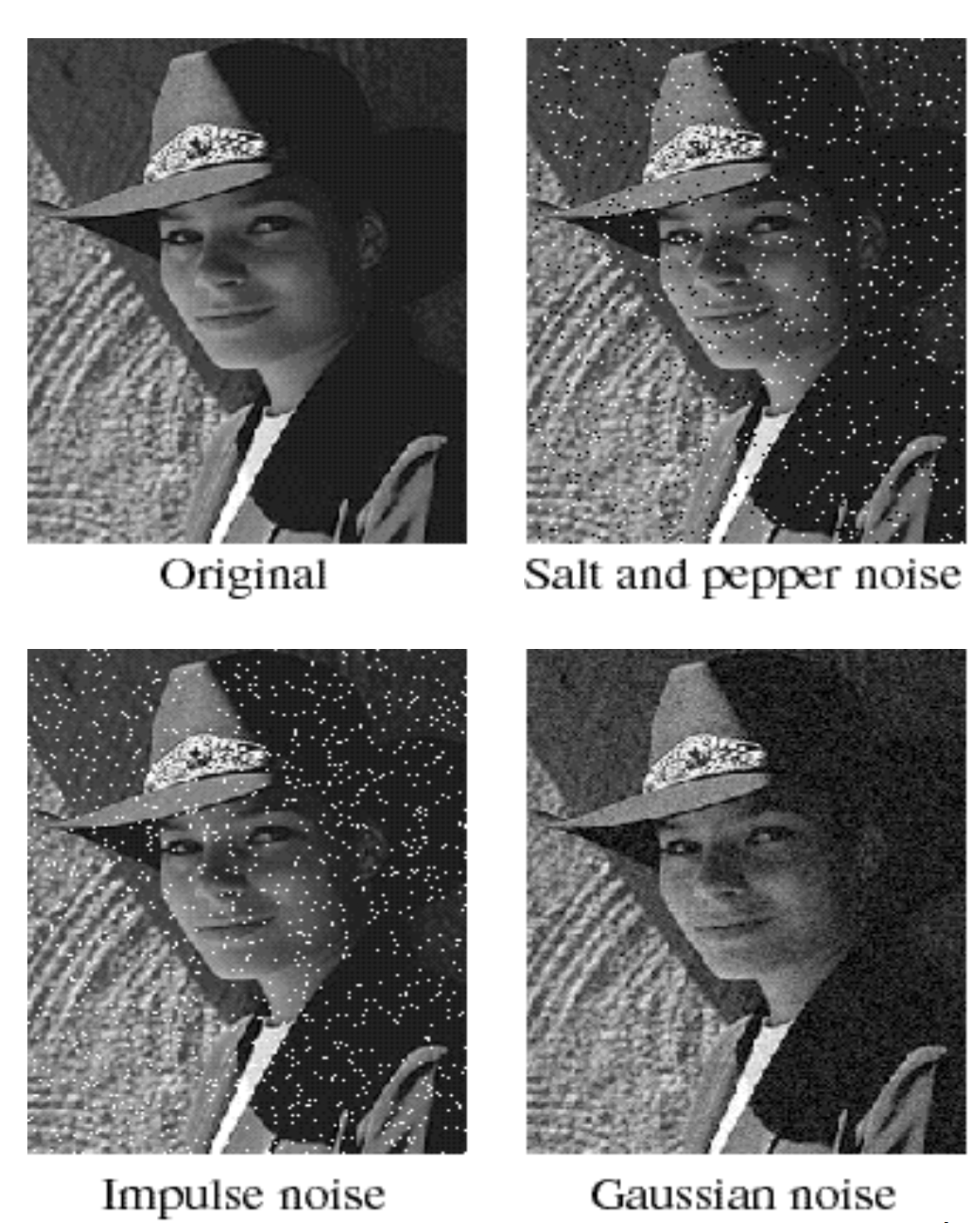
**Effigy 2. original and noise-introduced images. slide credit: [1], [3]**

Table salt & pepper noise indicates the random occurrences of black (pepper) and white (common salt) pixels across the image, significant some randomly selected pixels are set as black or white.
In dissimilarity, Impulse noise means the random occurrences of white pixels merely.
Lastly and importantly, Gaussian noise is the well-nigh commonly observed type of noise. Information technology introduces variations in intensity drawn from a Gaussian distribution. In other words, each pixel intensity in the image is modified by a random variable drawn from Gaussian distribution.

Fig iii illustrates the effect of Gaussian noise. The lower panel (graphs) shows the pixel color values 𝑓(𝒙, 𝒚) in the red horizontal line in image. By comparison the two pixel-intensity graphs, one can find the result of Gaussian racket: The pixel-colour values behave more like a zigzag design and they vary around true values.

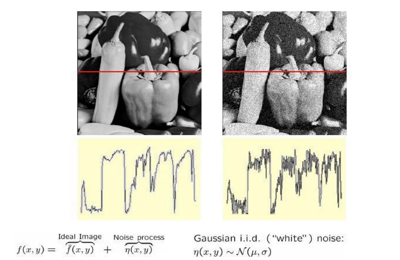
Figure iii. Analogy of the Gaussian racket. Left panel: original image with its pixel intensities in the reddish horizontal line. Right panel: image with additive Gaussian racket. slide credit: [one], [2], Martial Hebert

Note that the basic supposition here is that noise is "i.i.d" (contained and identically distributed)

3. Solution to reduce the noise

We want to find a way to reduce the dissonance in epitome. In other words, our goal is to reconstruct the given noise-introduced paradigm such that the dissonance level in image decreases. In order to achieve the goal, two fundamental assumptions are made.

Pixels in the prototype are expected to be similar their neighbours (having like pixel intensity)
Noise is independent from pixel to pixel (i.i.d)

3.i Moving Average Filter

**Figure iv. Illustration of the moving average, from [i], [3]**

Fig 4 presents how the moving boilerplate in second epitome works. Allow 𝐅 denotes the given image with two dissonance pixels, which are marked with yellow box (black pixel in the eye and white pixel in the depression-left corner), and 𝐺 indicates the filtered paradigm. The flow of moving average in Fig 4 is from left to right and from superlative to lesser panel.

What it does in Fig iv is that compute the mean of ix-pixel intensities in the reddish box (window) of 𝐅 then place it in 𝐺. Mathematically, this process can be represented as follows:

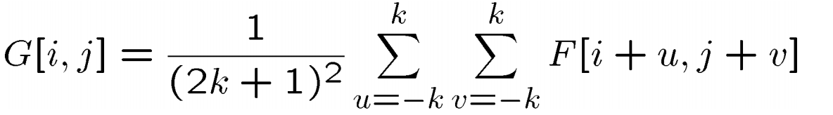
where two𝐤+1 denotes the window size in paradigm 𝐅. By doing so, the isolated noise pixels (in yellow boxes) and difficult borders (orange windows) in (4) of Fig 4 get shine out.

Note that averaging yields the smoothing! We will see why this smoothing is important in filtering in the side by side affiliate.

The topic of this article is "FILTER", and thus, one might enquire:

What is the filter of moving average in Fig 4 and Eq 1 ?

To respond this question, we need to know the correlation and convolution.

3.two Correlation

Let'southward start with the correlation. The mathematical definition of correlation is every bit follows:

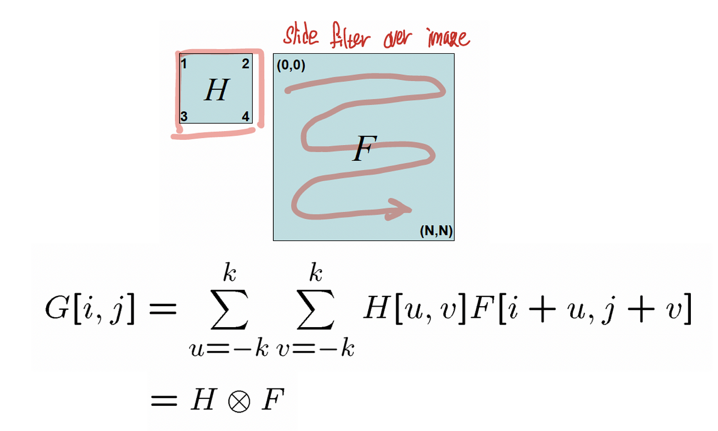
**Figure v. Definition and illustration of the correlation, from [i], [2]**

The correlation replaces each pixel of paradigm 𝐅 by a weighted sum of its neighbours, and such weights are determined by the filter H , which is also named "kernel" or "mask".

Doesn't the equation in Fig 5 ring whatever bell?

By setting H[u,v] for all u and five equally ane/(2k+i) ², nosotros obtain the Eq i of moving average. Therefore, we constitute the filter H, which is called the box filter, for moving average!

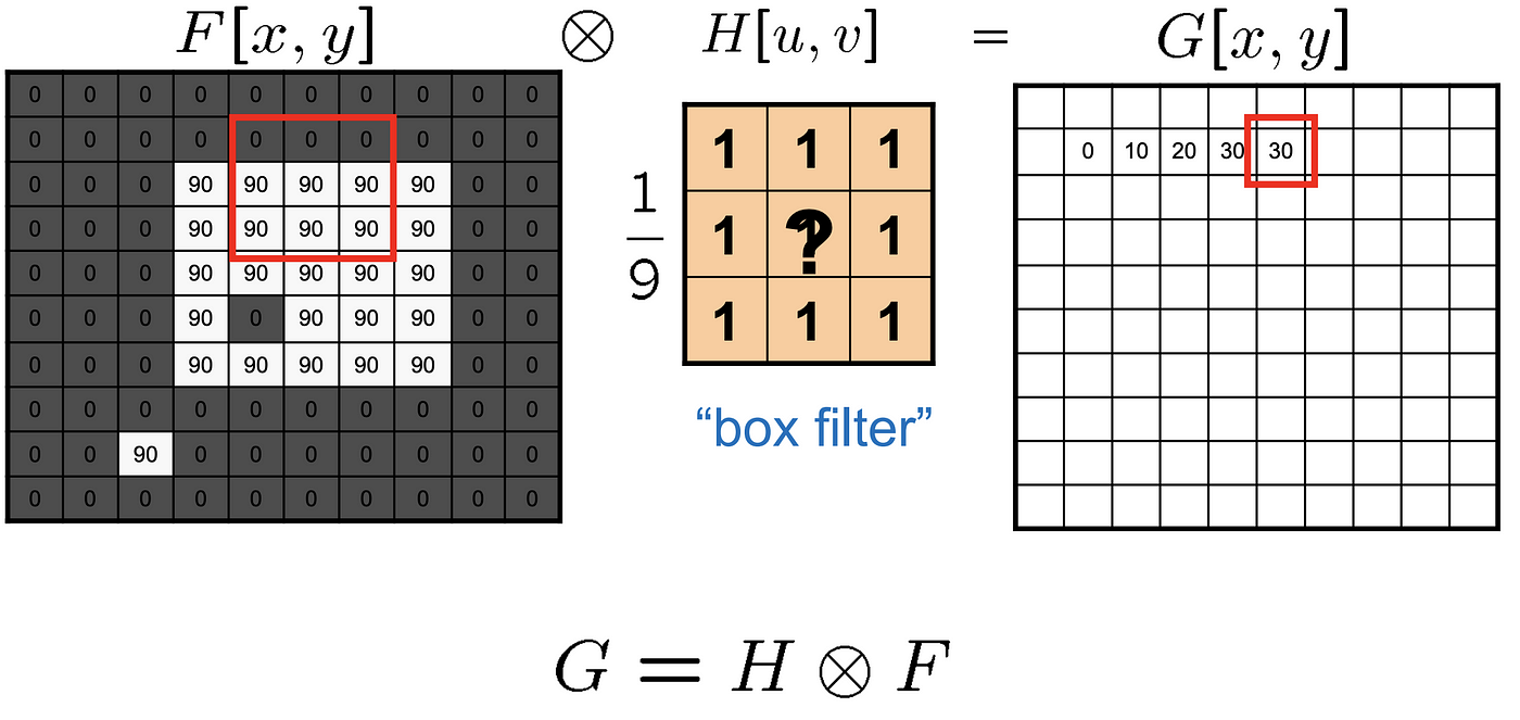
Higher up image illustrates the moving average with box filter when k = i.

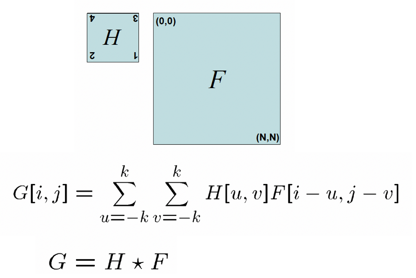
3.3 Convolution

Convolution is similar to the correlation, except for but one but significant difference. It flips the filter in both dimensions (right to left and lesser to superlative in case of 2D filter). And and then it applies the correlation. In curt, convolution is the combination of the filter flipping and correlation. Fig 6 illustrates this.

**Figure six. Definition and illustration of the convolution, from [1], [two]**

three.iii.one Properties of Convolution

Hither, I note some important and commonly used properties of convolution. Please take a closer await into each property and endeavor to bear witness them yourself.

f ⭑ (k × thousand) = k × (f ⭑ 1000)
f ⭑ (g₁+g₂) = f ⭑ g ₁+ f ⭑ g₂ : linearity
H[-u, -five] = H[u, five]: when flip( H ) = H , so correlation = convolution by definition.
f ⭑ (k ⭑ g) = (f ⭑ g ) ⭑ grand : Associative
f ⭑ g = g ⭑ f : Commutativity

And there are three more properties: Differentiation, Separability of second convolution, and nigh importantly the relationship betwixt convolution and Fourier transform . We volition take a deeper wait into them when we larn the Gaussian filter in the side by side chapter.

4. Decision

Nosotros have gone through the definition of terms: filter and noise, the idea of very basic filter: moving average. Also the correlation and convolution with their properties. Base on them, the next chapter will deal with more than avant-garde concepts: what is Gaussian smoothing (filtering), what is the effect of convolution in the frequency domain and what needs to be considered while filtering.